Mobile robot simulation with SciPy ODE solver and dynamic model (0–20 points)
Goal
Extend the mobile robot simulation by introducing:
- a dynamic model of the robot,
- numerical ODE solving using SciPy,
- a feedback controller for trajectory tracking.
The project should simulate realistic motion of a mobile robot in a 2D environment using ROS 2.
Description
Create a ROS 2 based simulation system for a mobile robot moving on the XY plane.
The robot motion should be calculated numerically using the SciPy ODE solver (solve_ivp).
Unlike the previous kinematic-only model, the robot should now include:
- mass,
- rotational inertia,
- linear damping,
- angular damping.
The robot should accelerate and decelerate realistically under the influence of applied forces and torques.
Additionally, the system should include a feedback controller responsible for:
- trajectory tracking,
- waypoint navigation,
- generating control inputs for the robot.
Robot state
The robot state is defined as:
X=[x,y,\phi,v,\omega]^Twhere:
x, y— robot position,φ— robot orientation,v— linear velocity,ω— angular velocity.
Robot model
The robot motion is described by the following differential equations.
Kinematic equations
\left\{\begin{array}{rcl} \dot{x} & = & \cos{\phi}\cdot u_1,\\ \dot{y} & = & \sin{\phi}\cdot u_1,\\ \dot{\phi} & = & u_2,\end{array}\right.Dynamic equations
Linear
m\dot{v}=F-bv
Angular
I\dot{\omega}=\tau-c\omega
where:
m— robot mass,I— rotational inertia,F— driving force,τ— steering torque,b— linear damping coefficient,c— angular damping coefficient.
Complete ODE system
\dot{X}= \begin{bmatrix} v\cos\phi \\ v\sin\phi \\ \omega \\ \frac{F-bv}{m} \\ \frac{\tau-c\omega}{I} \end{bmatrix}The system should be solved numerically using:
scipy.integrate.solve_ivp,- RK45 method (default),
- fixed simulation update step.
Control system
The robot should include a feedback controller responsible for trajectory tracking.
The controller should:
- compute position and orientation error,
- generate force and torque commands,
- navigate through a sequence of waypoints.
Position and heading error
Distance to target:
e_d=\sqrt{(x_t-x)^2+(y_t-y)^2}Desired heading:
\phi_d=\operatorname{atan2}(y_t-y,x_t-x)Heading error:
e_{\phi}=\phi_d-\phiProportional controller
Linear control:
F=K_p^d e_d-K_v vAngular control:
\tau=K_p^{\phi} e_{\phi}-K_{\omega}\omegawhere:
Kp— proportional gains,Kv— linear damping gain,Kω— angular damping gain.
Waypoint navigation
The robot should navigate through predefined waypoints, for example:
waypoints = [
    (2, 0),
    (2, 2),
    (0, 2),
    (0, 0)
]
The robot should switch to the next waypoint after reaching the current target within a selected tolerance.
The diagram shows an example system
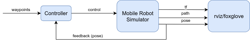
Requirements
The simulation should be implemented as a ROS 2 package.
The system should:
- simulate the robot motion in real time,
- publish robot pose,
- publish robot path,
- broadcast TF transforms,
- visualize motion in RViz or Foxglove.
The system should publish:
/pose— robot pose (geometry_msgs/PoseStamped),/path— robot path (nav_msgs/Path),
The system should also broadcast:
world -> base_linktransform using TF2.
Launch system
Create a Python-based launch file:
ros2 launch mobile_robot_sim simulation.launch.pyThe launcher should:
- start all nodes,
- load YAML configuration,
- optionally start RViz.
Remarks
-
Assume that the robot is moving on the XY plane and z is equal to 0.
-
Assume that at the beginning robot is placed in point (0,0,0).
-
The simulated robot should move in a meaningful way, for example, along a square (not a circle, as the control signals should not remain constant).
-
Create a new ROS 2 package for your robot simulation project.
-
Document code.
Example of ODE solving with SciPy – solve_ivp
from scipy.integrate import solve_ivp
import matplotlib.pyplot as plt

# RHS of the ODE dot(x) = f(t, x, p), where
# t -- time
# x -- state
# p -- parameter
def f(t, x, p):
  return -p * x

T = [0, 10] # Time horizon
x0 = [2] # Initial state
p = 0.5 # Parameter

# Solve
sol = solve_ivp(f, T, x0, args=[p])

# Plot the solution
plt.plot(sol.t, sol.y[0], label='x(t)')
plt.title('ODE Solution')
plt.xlabel('Time (t)')
plt.ylabel('State (x)')
plt.legend()
plt.show()
SciPy installation (if necessary)
pip install scipyOptional extensions
Additional points may be awarded for:
- dynamic parameter updates,
- lifecycle nodes,
- URDF visualization,